3D prominence formation Author: Jack Jenkins
In the well-received previous work that we detailed here, we used the open-source MPI-AMRVAC code to study the formation and evolution of coronal condensations (cool plasma) within a 2.5D flux rope. By constructing distance-time representations of these simulations, and converting the primitive variables (pressure, temperature) into information relating to the emission/absorption of the associated plasma, we were able to approximate the appearance of the small-scale evolution of solar filaments and prominences. Since then, we have been working hard on bringing these simluations to life, that is, bringing them into the real 3D world. In this post, we’re going to highlight the tools used, and associated results, to decode the simulation from a bunch of numbers in a matrix to finally resemble the images of the solar atmosphere that are captured on a daily basis. If you’re interested, however, then the more technical details involved in the process of creating the simulation itself are available here.
If you imagine a three-dimensional volume, a region of space, that you can split up into little cubes then you have a pretty good representation of the raw output of our simulation. The more cubes we split this volume into, the higher the resolution that we are dealing with i.e., we can see smaller and smaller details. Naturally, anyone working with simulations wants to make it so that they can see all of the intricate details within whatever physical process they’re approximating with computer code. Indeed, a great deal of focus within the simulation community centers on improving computational efficiency, and this is because if you increase the resolution (think of it as increasing the number of little squares) then it takes longer to complete a simulation as it has to compute more ‘things’, as it were. The 3D simulation we have completed is one of the highest resolution simulations of solar filaments/prominences that has ever been completed. Now this highlights the computational efficiency of MPI-AMRVAC, for one, but there’s another consideration here.
All of that information has to be stored, right? And once it’s stored, it has to be opened by a program so you can check the results, analyse them, and create plots and movies etc. For the 2.5D simulations (imagine a slice comprised of a single 2-dimensional row + column of information) that we spoke about earlier, this wasn’t so complicated as each individual file, corresponding to a single timestep, contained not much more than ~ 2 GB of information. If you’re even remotely familiar with modern computer architecture then you’ll know that this is relatively trivial to load into RAM and access with whichever program is your favourite. Of course, this becomes slightly more complex when you have, say, 700 files that you want to process - but then the processing simply becomes a matter of time. If we now fastforward to our new 3D simulations, each file is approximately 10 times larger (32 – 45 GB) and whilst some big computers might be able to load that all into RAM it will be extremely slow to process, and this is just for a single file out of the potential 700… So how did we overcome this? yt-project is the python library at the heart of our post-processing tools and the incredible developers that maintain this framework are to thank for making simulations like ours feasible. Afterall, what’s the use of such an immense simulation if we can’t see the results? In short, instead of reading the entire simulation into the RAM in one go, the structure of a single file is mapped such that only the reference information is stored in the RAM. Assuming I want to take a slice of the simulation and take a look at the density, the stored framework tells the ram exactly where in the file (i) the density information is stored and (ii) where the information about the density in the slice I want, is stored. This might seem like a small distinction but it is fundamentally different from reading all the data in and showing only what I ask for. The important result is that I can view a slice within my simulation in a fraction of a minute, rather than after some hours.
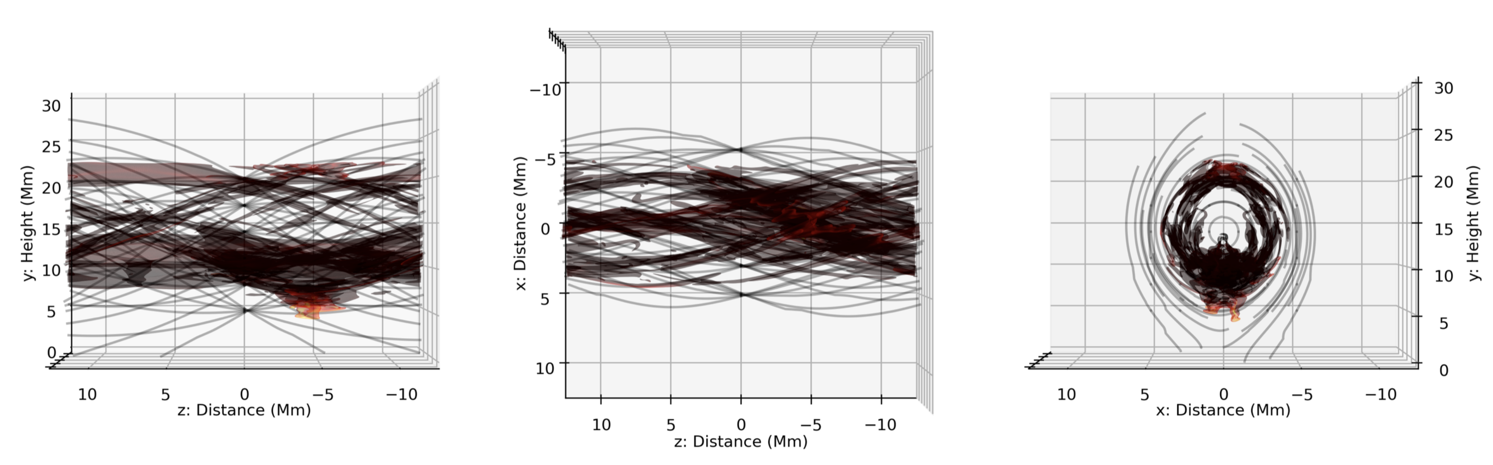
Once the data can be readily accessed, manipulating it is far more trivial. This is further facilitated by the yt-project framework, be that the many integrated or definable derived fields, or the methods e.g., volume rendering. And so without further ado, the first movie presents a volume rendering of the simulated 3D solar prominence. This particular snapshot is at the very end of the simulation i.e., once the flux rope has been constructed and the condensations have formed and evolved a short while (~ 15 minutes). Those with an astute eye will notice that this visualisation resembles a collection of coloured isocontours with varying degrees of transparency, when in fact a transfer function is at play that gives you far more freedom in specifying the contours, colours, and alphas.
Now, such a rendering can tell us a lot about the internal structuring of solar prominences in relation to their magnetic field. For example, with prior knowledge of the structure of the magnetic field within the simulation, we can say that the prominence material is largely bound to the magnetic field i.e., the magnetic field guides the evolution of the solar plasma. Now this isn’t a new conclusion, but it’s nice to see it so clearly in this example.
When we observe solar filaments and prominences within the solar atmosphere, however, we aren’t able to say exactly what the magnetic field structuring is because we are yet to invent a method for directly observing it within the corona. Fortunately, we can just about infer the magnetic field within the prominence plasma, using something called the Hanlé effect, and this gives us some hints as to the conditions that we expect there. Whilst a direct comparison of the magnetic environment isn’t possible, a visual comparison between what we observe in the solar atmosphere and what we have created with our simulation is far more trivial. In practice, this is where the derived fields of yt-project come into play once more. We begin by assigning emission and absorption properties to a single voxel, using a series of well-known equations based on the physical quantities available within the simulation. We then also make use of the arbitrary-perspective projection framework of yt-project to construct a synthetic images of the 3D simulation domain that then correspond to images taken daily by state-of-the-art space-based telescopes. Below, is one of these such synthetic representations of the simulation domain, demonstrating both the axis-aligned and arbitrarily-positioned options. These images are made to represent the images taken by the Atmospheric Imaging Assembly on board the Solar Dynamics Observatory (specifically the 171 angstrom passband) and the groundstation obsevrations of the Global Oscillation Network Group (specifically the Hydrogen-Alpha spectral line core).